Randomization Coverage Verification
Obtaining the tool The coverage verification tool is a standalone offline program. It is not currently distributed with the platform, and it does not modify existing datasets when run. To request it, please contact us at aide.support@advantech.com.
Purpose of verification
The randomization range is the central setting of SDG, but having configured it is not the same as the data having actually spread out. Neither of the two signals the platform provides — the success rate and single-episode playback — answers that question: the success rate reflects only whether the motion completed, playback reflects only whether that episode looks normal, and neither describes the shape into which the initial object positions of the batch as a whole are distributed.
This judgement should not rest on visual inspection. Playing back a hundred episodes one by one leaves no impression beyond "it seems to have spread out", while the most common failure is precisely this: eighty percent of the objects fall within a small region at the centre of the frame and not one episode reaches the four corners. Every episode of such a dataset appears normal on playback; the anomaly is visible only in aggregate.
This tool performs a single function: it plots the initial object positions of the entire batch. The scatter plot shows the distribution, the heat map shows the density, and together they establish the extent of space the batch actually covers.
When to run it
The tool itself is of limited technical complexity; its value lies in the cost it averts. Generating a hundred episodes takes considerable time and training takes longer. Where the randomization range is set too narrowly, no stage along that path reports an error:
| Stage | What is observed | The actual situation |
|---|---|---|
| Generation | A near-perfect success rate | Because every object sits where the arm reaches most easily |
| Spot check | Every episode is normal | Because each episode genuinely is normal |
| Training | The loss curve converges cleanly | Because there is only one situation to learn |
| Physical inference | The slightest offset defeats the grasp | Because the model has never seen that position |
The problem surfaces only at the last row, by which point the full cost of generation and training has been paid. This is the same principle stated in the simulation environment chapter — confirm before scaling up: confirmation costs minutes, the failure to confirm costs the whole batch.
The position of this procedure is therefore: after generation is complete, and before export and training.
Preparing the images
The tool reads images, not dataset files. What is required is the first top-camera frame of each episode — the frame in which the arm has not yet moved and the object rests at its randomized initial position.
The folder structure is as follows:
first_frames/
├── 20260506_0947/          ← session (a timestamp name is recommended)
│   ├── demo_0_cam_top.png
│   ├── demo_1_cam_top.png
│   └── ...
├── 20260506_1040/
└── 20260506_1132/
| Item | Requirement |
|---|---|
| Filename format | demo_<number>_cam_top.png; the number is used to label the plot |
| Folder structure | One folder per session; PNGs may also be placed directly in the root |
| Camera | Top view. A side view cannot represent a planar distribution and is unsuitable |
| Target object | A red cube (for other colours, see Adjustable parameters) |
The purpose of separating sessions is comparison between batches. In practice generation is rarely completed in a single pass: one batch is run, the range is adjusted, and a further batch is run. Once separated into folders, the scatter plot colours each batch differently, so that whether the adjustment produced a wider distribution can be read directly rather than inferred from a single merged result.
Running the tool
pip install opencv-python numpy matplotlib pillow
python app.py
The run produces cube_distribution.png in the working directory, and the terminal lists the detected coordinates frame by frame:
── 20260506_0947 ──
  20260506_0947 [ 0] (412.3, 288.7)
  20260506_0947 [ 1] (395.1, 301.2)
  20260506_0947 [ 2] NOT DETECTED
  20260506_0947 [ 3] WARNING: homography failed, using raw
Two messages warrant attention:
| Message | Meaning | Handling |
|---|---|---|
NOT DETECTED | No red region was detected in that image | One or two occurrences may be ignored; large numbers indicate an unsuitable colour threshold, see Adjustable parameters |
homography failed, using raw | Camera-angle correction failed; raw pixel coordinates are used instead | A small number is acceptable; large numbers indicate insufficient background features, see Camera-angle correction |
Interpreting the output
The output consists of two plots side by side, sharing a single reference image as their background.
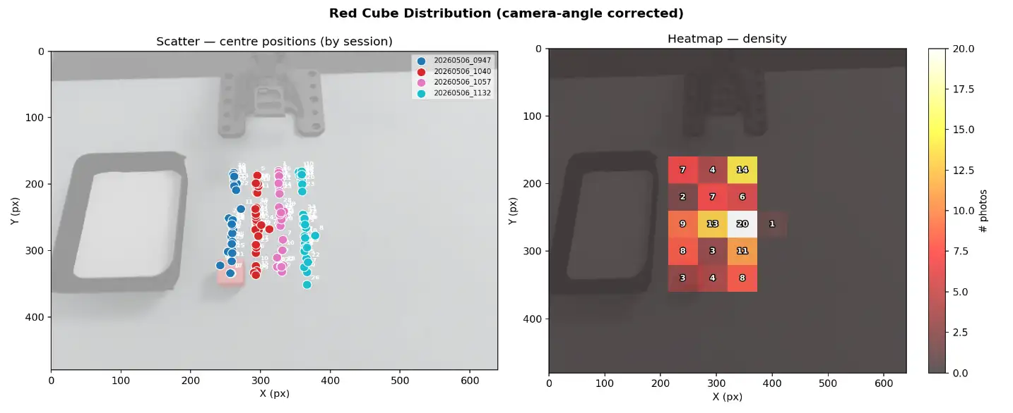
Scatter plot
Each point is the centre position of the cube in one image, coloured by session, with the demo number labelled alongside.
What is to be read is the shape, not the individual point. A sound distribution should broadly fill the intended working area rather than cluster into a small patch or align into a line.
The labelled numbers serve traceability: where a point falls in isolation near a corner, its number may be noted and that episode played back, which in most cases reveals a failed or anomalous episode.
Heat map
The image is divided into a 12×12 grid, the number of points falling in each cell is counted, and the density is represented by shade (black → red → white), with the actual count printed in the cell.
At larger data volumes the scatter plot overlaps itself: with a hundred points superimposed, a central region of ten points cannot be distinguished from one of forty. The heat map exists for this purpose.
Three shapes require action:
| What the plot shows | What it represents | Corresponding action |
|---|---|---|
| One central cell with a notably large count, surrounded by zeros | The randomization range is too narrow, equivalent to duplicating one episode a hundred times | Widen the randomization range of the cube and the box |
| A broadly even distribution, slightly lighter at the edges | Normal | No adjustment required |
| A pronounced bias to one side, with the other side blank | The centre value of the randomization range is offset; this is not a question of width | Check the virtual-physical alignment |
The last case merits particular attention. An excessively narrow range and an offset centre value are indistinguishable by success rate, yet their remedies are opposite: the one requires widening, the other requires moving the centre. Only the distribution plot separates them.
A worked reading
The plot above is an actual output: four sessions, 120 episodes in total, at a frame size of 640×480. Read by the method above:
First, the extent of the distribution. All points fall within a region of roughly x 240–380 and y 175–345; of the 144 cells only 16 contain data, less than a ninth of the frame. The hottest cell of the heat map holds 20, meaning that a sixth of the entire dataset falls within 1/144 of the frame. By the table above, this is the classic case of an excessively narrow range.
Second, the colours of the scatter plot. The four sessions each form a vertical band, arranged left to right with almost no overlap. This means that the variation in x within any single batch is small, and that the apparent width of the whole is produced by the differing centre values of the four batches taken together.
This distinction changes the remedy:
| If it is judged that | The actual situation is | The correct action is |
|---|---|---|
| The four batches together already cover the area | A model trained on any single batch has seen only one narrow band | Widen the randomization range of the individual batch, rather than running further batches with shifted centre values |
Assembling coverage from multiple batches with shifted centre values does not have the same training effect as setting a wide range within one batch. The former is a superposition of several narrow distributions, leaving gaps of uneven density between them; only the latter provides the continuous variation the model requires.
Third, outliers and blank regions. The isolated 1 at the right of the heat map corresponds to the lone point at the far right of the scatter plot; noting its demo number and playing that episode back will usually reveal anomalous data. The blank area at the left, where the box stands, is by contrast correct — the cube is never generated inside the box.
A blank cell is not necessarily a deficiency. Where the region in question lies beyond the reach of the arm, the absence of data there is the correct result. The question to ask is not whether the frame has been filled, but whether the range in which the workpiece will actually appear in production has been covered.
Camera-angle correction
Where the randomization range of the top camera has also been enabled (that chapter recommends a more conservative setting than for the object, but not zero), the camera position differs slightly in every episode, and a single physical position falls at different pixel coordinates across frames.
Plotting the raw pixel coordinates of all episodes together therefore measures the variation of the object plus the movement of the camera, and the distribution appears wider than it is. Since what is to be judged is precisely how wide the distribution is, this error falls exactly where it does most harm.
The tool handles this as follows:
demo_0of the first session is taken as the global reference frame- Each image is matched against the reference frame using ORB features, with the red cube region masked out beforehand (dilated by 20 px) so that the moving object itself does not disturb the alignment
- A homography matrix is estimated by RANSAC
- The detected centre point is mapped back into the coordinate system of the reference frame
What is then measured is the positional variation of the object alone.
Failure cases: where fewer than eight feature matches or fewer than six RANSAC inliers are found, that image falls back to raw pixel coordinates and a warning is printed. A few such fallbacks do not affect the overall reading; large numbers usually indicate an excessively clean background — a plain-coloured table offers insufficient texture for matching. Affixing something patterned at the edge of the field of view (tape, a label, a graduated sticker) resolves this, and such markers are also of use when repositioning the camera later.
Distinction from camera calibration Deriving camera pose from feature points, as described in this section, is a different matter from camera calibration. Calibration measures the absolute position and orientation of the camera and stores them to a file; what is done here is only a relative alignment of each image into a common coordinate system, discarded after use. Neither substitutes for the other.
Adjustable parameters
Four values may be adjusted, at the top of the file and within main():
| Location | Variable | Default | When to adjust |
|---|---|---|---|
| Top of file | FRAMES_DIR | first_frames | Images are held at another path |
| Top of file | OUTPUT_PATH | cube_distribution.png | The output is to be saved elsewhere |
main() | bins | 12 | A finer grid is required for a large dataset (a larger value gives smaller cells) |
make_red_mask() | HSV range | See below | The target object is not red, or the lighting on site is dim |
On bins: the default of 12×12 is chosen so that the cell counts remain legible on screen. Once the distribution is confined to a small region, however, 12 cells are too coarse to reveal its internal structure — where the example above occupies only three or four cells in width, a value of 20–24 is required to determine whether that region is internally uniform or contains a smaller hot spot of its own.
Changing the colour or accommodating the lighting is the most common modification. Red spans both ends of the HSV hue circle, so the program uses two masks:
m1 = cv2.inRange(hsv, (0, 100, 80), (10, 255, 255))      # 0–10°
m2 = cv2.inRange(hsv, (160, 100, 80), (180, 255, 255))   # 160–180°
The three values are hue, saturation, and value. Another colour requires only one mask, with the hue range adjusted; where dim lighting on site produces large numbers of NOT DETECTED, the lower bound of value (80) should be reduced.
detect_red_cube() further applies an area threshold of area < 50 to filter out isolated noise. Where the cube is particularly small in frame and is filtered out in error, this value should be reduced.
Limits of applicability
Its boundaries should be clear, so that its conclusions are not used to answer questions it cannot address:
| Limit | Description |
|---|---|
| It measures pixels, not centimetres | The output coordinates lie in image space. Relative density may be compared; they do not correspond directly to centimetres. Conversion requires camera calibration |
| Only the largest red region is taken | A second red object in frame may be mistaken for the target. Confirm before running that no other object of the same colour is in view |
| Only the initial position is examined | What is verified is whether the starting points are spread; trajectory quality is not covered and must still be confirmed by playback |
| Only top-view images are accepted | Distribution is a planar concept and cannot be measured from a side view |
| The z axis and rotation are invisible | A top view reflects only x and y. Where the height and z rotation of the cube are also randomized, this plot cannot show whether those two took effect |
The last point bears expansion: what this tool verifies is the two most important and most commonly misconfigured dimensions of the randomization range, not all of them. It is an inexpensive check, not a complete guarantee of quality.
Checklist
Before running
- The first top-view image of each episode has been extracted, named
demo_<N>_cam_top.png - Separate batches have been placed in separate session folders
- No other object of the same colour as the target is in the field of view
- Where the target is not red, the HSV range in
make_red_mask()has been adjusted
When reading the output
- The counts of
NOT DETECTEDandhomography failedare within acceptable limits - The distribution in the heat map covers the region in which the workpiece will actually appear in production, rather than merely filling the frame
- The width of the distribution derives from the randomization range of a single batch, not from several batches with differing centre values
- Where the distribution is biased to one side, the virtual-physical alignment has been checked rather than the range simply widened
- Outliers in the scatter plot have been noted by number and confirmed by playback
After confirmation
- Export and training proceed only where the distribution meets expectations; otherwise return to the simulation environment, adjust the settings, and generate again
Once the distribution meets expectations, proceed with model training. This check does not make the model more accurate; its function is solely to establish the extent the batch actually covers before the cost of training is paid. A model can learn no more variation than it has seen, and this plot shows precisely how much it has seen.
Next: Dataset management.